ATtiny Development Board

I recently had to program an ATtiny85. As I was developing, I got tired of repeatedly wiring the connections between a 6-pin ISP socket and the ATtiny, and wanted something more permanent. I found myself sucked into Eagle CAD and this is the result. It has everything necessary to program 8-pin and 14-pin Atmel microcontrollers ATtiny25, ATtiny45, and ATtiny85.

The gerber files are available at my Github repository.

The circuit is quite simple – it connects the ISP pins 5V, GND, ~RST, MISO, MOSI, and CLK to the corresponding pins on the ATtiny, allowing for easy programming with any ISP programmer. It breaks out the power pins of either board to a pair of pins next to the ISP socket, and it breaks out and labels all the other pins of the ATtiny along the side of the board. For use in development, the programmed chip can be powered through the power-input pins near the 7805 voltage regulator (give it 7-15V); in this configuration the 10K resistor pulls up the ~RST pins to enable the ATtiny chips to operate.

ATtiny_dev_board_schematic

ATtiny_dev_board_board

Updating some, but not all, old technology

Lightning strikes. It struck near me, and fried a component of my old X10 home-control system.

X10 is a power-line-based communications network. Data is sent (slowly) over the house power lines by injecting a 120 kHz signal into the 60 Hz AC signal just after the zero-crossing of that signal. One bit per cycle is sent by either adding or withholding a short pulse of the 120 kHz.

System Description

X10 devices are either plugged or wired into the house power lines. Each device has an address, not necessarily unique, which consists of a house code A-P and a unit code 1-16. The original design intent was to have each house in a neighborhood choose a unique house code, to prevent signals from the neighbors from controlling one’s own devices.

The data sent over the power lines corresponds to commands like “A03 AON”, which says to turn on any device with house code A and unit code 3.

    I had been using a TW523 interface which provides:

  • a logic-level zero-crossing synchronization signal
  • a logic-level output which indicates when a 120 kHz carrier is present on the power line
  • a logic-level input which causes the generation of the 120 kHz carrier.

It was controlled by an old Arduino which passed commands between the TW523 and a UDP socket using an Ethernet shield.

A Perl script on another computer provided the intelligence – receiving messages from the X10 system and an auxiliary RF control box, from my MQTT message broker, and from a Perl scheduler.

The Event

A recent thunderstorm provided my next-door neighbor some excitement when a bolt hit his chimney. It provide me with something to do, too…

It fried my TW523.

I subsequently found that the devices aren’t manufactured anymore. Fortunately, Jeff Volp produces a plug-compatible replacement, the XTB-523. I’m not yet using its extended capabilities, but am enjoying the higher reliability produced by its higher-power signals.

The Project

However, being a geek, I had to make other improvements to my system.

I didn’t like the power consumption of the old Arduino and its Ethernet shield – the Arduino’s voltage regulator was always quite hot, and I was afraid it would cook itself. I also didn’t like the solderless breadboard I had cobbled together 20 years ago as an electronics newbie – it was a mess.

So I grabbed a spare Adafruit Huzzah ESP8266 breakout board and went to work on the software. [ I will upload that to my Github account once I figure out why it’s telling me hundreds of my files have changed and I should do a pull but it won’t let me anyways and … wah, wah, wah ]

I also needed to create a better hardware setup – I wanted to plug the Huzzah into a board with its own voltage regulation, level shifting, and an RJ11 jack for the phone wire to connect it to the XTB-523. I entered the schematic into Eagle and laid out the components as if I were going to produce a PCB. I do this even when I’m going to hand-wire a circuit board, just to the point of laying out the components but not laying out the traces. I generally also create and record a color code for the wires, which will help me in future debugging.

This time around I also remembered to add some test points onto the board. I have a 4-pin header for the power (Vcc, 5V, 3.3V, and GND) and one for the 4 connections to the XTB-523.

After some major troubles with the software, I got it all to work. The main software trouble was a bug in the X10 library. I was getting an ESP8266 fatal exception when I enabled receiving. As I tried to create bread crumbs ( Serial.print statements ) and follow them back, I found that the problem arose in an object method that was called from an interrupt service routine (ISR). Now, it’s a really bad idea to do anything in an ISR that takes any significant time at all, because other interrupts want to be serviced, too, and they can’t while one ISR is in control. Print statements take a really long time ( from the perspective of a computer ), so trying to put them in confounded my search for enlightenment. Eventually I got frustrated enough to put some print statements outside the ISR and learned that the object’s .cpp file had to define an object pointer ( so the ISR could call an object method ), but that it wasn’t initialized to point to anything. When you try to dereference a null pointer, bad things happen. Once I found that, I was past the hump.

I almost said, “Once I found that, I was home free.” But I wasn’t. I still had (gasp!) bugs in my own code. They were, however, readily found and fixed.

Now everything works. <contented smile>

References:

Experiment with CircuitPython, Jupyter, and WordPress

I’m trying to embed a Jupyter notebook page as a blog post. I saved it as html, and copied an pasted that html below. I don’t think that’s the best way to do it.

We are exploring the Adafruit Metro M4 Express

Poking around, wanting to see if we can access the hardware timers, we set ourselves a problem:
We want to see how long it takes to update the NeoPixel’s color. Let’s start by exploring the time library:

In [1]:
import time
print ( dir ( time ) )
['__name__', 'monotonic', 'sleep', 'struct_time', 'localtime', 'mktime', 'time']
In [2]:
print ( time.time() )
946696312

So it looks like time.time() returns seconds since some fixed epoch – probably midnight, January 1, 1970, which epoch is a standard amongst Unix installations — but I haven’t checked this…

Next we’ll set up the NeoPixel

In [3]:
import board
import neopixel

pixel = neopixel.NeoPixel ( board.NEOPIXEL, 1 )

And now we want to see how many updates we get in one second. We don’t expect to get a very consistent number, because we’re not being really accurate with our timing.

In [4]:
t = time.time()
n = 0
while time.time() == t:
  # do nothing until we get a clock change
  pass
t = time.time()
while time.time() == t:
  n += 1
  pixel[0] = [ 2, 2, 2 ]
print ( n )
1032

A better way to time would be to extend the time interval:

In [5]:
durationOfTest_seconds = 5
secondsUsed = 0
numberOfIterationsCounted = 0

t_seconds = time.time()
while time.time() == t_seconds:
  # wait, doing nothing, until we get a clock change
  pass

t_seconds = time.time()
while secondsUsed < durationOfTest_seconds:
  pixel[0] = [ 2, 2, 2 ]
  numberOfIterationsCounted += 1
  if time.time() != t_seconds:
    secondsUsed += 1
    t_seconds += 1
print ( numberOfIterationsCounted / durationOfTest_seconds )
1021.4

Better yet would be to keep running the test until the standard deviation dropped to less than 1. We’ll calculate the variance as v(x)=E(x2)E(x)2

v(x)=E(x2)−E(x)2

E(x2)E(x)2=x2/n(x2/n2)=(x2nx2)/n2

E(x2)−E(x)2=x2/n−(x2/n2)=(x2∗n−x2)/n2 


or, because this is sample variance,

E(x2)(E(x))2)=x2/nx2n2=x2nx2n(n1)

E(x2)−(E(x))2)=x2/n−x2n2=x2∗n−x2n∗(n−1) 

In [ ]:
import math

stdevUpperLimit = 20
stdev = stdevUpperLimit + 1

# statistical moments of inertia
n = 0    # number of events summarized
x = 0    # sum of values
x2 = 0   # sum of squares of values

while stdev > stdevUpperLimit:  # keep testing until criterion matched
  
  t_seconds = time.time()
  while time.time() == t_seconds:
    # wait, doing nothing, until we get a clock change
    pixel[0] = [ 0, 0, 0 ]
  
  numberOfIterationsCounted = 0
  t_seconds = time.time()
  while time.time() == t_seconds:
    pixel[0] = [ [ 5, 0, 0 ], [ 0, 5, 0 ], [ 0, 0, 5 ] ] [ n % 3 ]
    numberOfIterationsCounted += 1
  # completed 1 test event; summarize statistics
  n += 1
  x += numberOfIterationsCounted
  x2 += numberOfIterationsCounted * numberOfIterationsCounted
  
  # calculate the mean and standard deviation of all the tests so far
  if n > 0:
    mean = x / n
    if n > 1:
      # variance = e(x2) - e(x)**2
      variance = ( ( x2 * n ) - ( x * x ) ) / ( n * ( n - 1 ) )
      stdev = math.sqrt ( variance )
      print ( "Mean: ", mean, "; Variance: ", variance, "; St Dev: ", stdev )
    else:
      # print ( "Insufficient tests for variance to be calculated" )
      pass
  else:
    print ( "No tests completed!" )

That one stinks — it runs forever if the stdevUpperLimit is set too low. So the next iteration needs to reverse everything – run n iterations of updating the NeoPixel and seeing how long that takes. We can measure elapsed time by using time.monotonic, which will give us a baseless value in ticks. Here we go:

In [6]:
numberOfIterationsCounted = 0
t_ticks = time.monotonic()
while numberOfIterationsCounted < 10000:
  pixel[0] = [ [ 5, 0, 0 ], [ 0, 5, 0 ], [ 0, 0, 5 ] ] [ numberOfIterationsCounted % 3 ]
  numberOfIterationsCounted += 1
t_final_ticks = time.monotonic()
print ( t_final_ticks - t_ticks )
7.80469

It looks like time.monotonic() is a count in seconds, but with high precision. The number we get, 8.8 or so, from the above routine is consistent with about 1ms updates which were the rough guesses of the previous program. But based on the variation across runs in the result – from 7.8 to 8.9 or so – coupled with the visual impression of there being unexpected pauses in the flashing of the NeoPixel, indicates to me that there’s some overhead in CircuitPython that makes it unwise to count on millisecond-scale timing accuracy.

EBD-USB+ Electronic Load – Testing Power Supplies and Batteries

I watched a video from Andreas Speiss reviewing electronic loads, and identifying one in particular called EBD-USB+ from zketech.com and purchased through Amazon or Banggood or wherever. The software is a little hard to find, but it’s available through this link. It comes as a .rar file, which you might need to unpack with 7-zip or Winzip. You will also need the driver.

The resulting Windows-only software allows one to test two categories of things: batteries, by allowing a set amount of current to flow and recording both current and voltage vs. time, and power supplies, by allowing an increasing amount of current to flow and recording voltage vs. current. The Speiss video explains really well.

Here are a couple of results I got while trying to locate a power supply capable of furnishing 5V at 2.1A to power a Raspberry Pi 3B. None of the five wall-wart power supplies really made the grade.

The worst of them, capable of providing only 4.72V at 2.1A

The best of them, the power supply that Adafruit sells and recommends for the Raspberry Pi. It provided 4.88V at 2.1A

Thoughts on serial communications

Maybe these issues have been solved in the past. I don’t think there is necessarily a very good solution, though.

The problem is that serial communications is imperfect. Characters get messed up in transit between two devices. When they do, that in turn messes up carefully thought out protocols, like “Capture characters in a buffer until you see the linend; then process the buffer as a single message.”

It’s a small problem if a message character gets corrupted. The message probably won’t make sense; that can be handled with an error message and some recovery process.

But what if the linend itself gets corrupted? Then your program won’t see it as the conclusion of a message, so it will continue capturing characters into the buffer. Then what? Two messages are now corrupted. Still no big deal. But then you have an increased risk of buffer overflow. ( You are checking to avoid buffer overflow, right? ) How to handle that? Flush the buffer and hope the next message is better? But the next message will most likely be broken, ’cause you probably flushed the buffer halfway through it, discarding the first part.

Finally, what do you do if the source goes away? There might be a partial message in the buffer. Should you have a timeout, after which you conclude that the source has crashed, and you need to flush the buffer so the next message that arrives, when the source has recovered, will not also be clobbered?

Think of these possibilities. Writing embedded software is not necessarily as simple as we’d like. But if we consider all the possible ways something can go wrong, and deal with them carefully, we can make software work well and robustly.

Teensy, touch sensing, and ESP8266 – via MQTT and Raspberry Pi

Whee!

I have a demo/development setup on a small breadboard which powers an ESP-01 ( the small, cheap, 8-pin breakout board for an ESP8266 chip ). In addition to being a programming board, it has 3v3 voltage regulation, a pot, a temperature sensor, a simple LED, and a WS2812 3-color LED. I have the installed ESP8266 running a program to subscribe to an MQTT broker and light the LEDs according to publications on a certain topic.

I’ve developed another small program which listens to a 115200 baud serial connection and accepts JSON messages which instruct it to connect to a WiFi, to publish values to an MQTT topic, or to subscribe to an MQTT topic. It is intended as a general-purpose glue service for an otherwise dumb microcontroller to communicate with remote telemetry.

I have also a Teensy 3.1, which supports capacitive touch sensing, interprets the values as control signals, and via the text-to-MQTT glue service publishes them, whence they will control the aformentioned LEDs. The program that does this is also on Github.

It all works, sort of. I’m considering it to be at the late-alpha stage of development.

Securing a Raspberry Pi IoT Gateway

I believe that the UMass IT policy forbids “rogue” WiFi gateways in order to prevent anonymous Internet access, so that nefarious actors can be identified.

I needed to create an IoT server for my lab, M5, and it needed to be accessible via WiFi. It also needed to have Internet access so that I could keep its Linux firmware up to date.

Securing it in accordance with the IT policy, and preventing tampering, required several actions:

  • disable forwarding of anything coming in from the WiFi port wlan0 to the ethernet port eth0
  • limit the user accounts to the minimum necessary
  • secure the privileged account “pi” by changing its password
  • disable remote root account login

I will address the first and the last of these actions.

Disabling of forwarding between the WiFi port and the ethernet port

There is a baffling mechanism called “iptables” that routes packets between the local host and its various network ports. Luckily, I had to deal only with the FORWARD chain. I simply had to flush the current rules out of the FORWARD chain

sudo iptables -F FORWARD

and add the one to reject forwarding:

sudo iptables -A FORWARD -i wlan0 -o eth0 -j DROP

Once the changes are made, they are made permanent by saving the tables into a rules file that is consulted at boot time:

sudo sh -c "iptables-save > /etc/iptables/rules.v4"

Disabling of remote root account login

Edit ( with root ) the file /etc/ssh/sshd_config and put the line

PermitRootLogin no

References:

Calculating the Axis of Nutation of my Solar Tracker

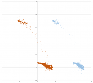
Following on the cluster analysis of the last post, I pairwise crossed (as in cross-multiply) the resulting cluster centers, and got three reasonably-close vectors after normalization. These were:

0 x 1: (-0.36, 0.93, -0.10)
0 x 2: (-0.23, 0.97, -0.06)
1 x 2: (-0.20, 0.97, -0.14)

While satisfyingly close, I wanted to do better.

Next I decided to take 1M random pairs of points from the raw data, cross and normalize these pairs, and then look at component-wise statistics. I ignored points within my arbitrary minimum separation of 0.5. The results were not only satisfyingly close, but also close to the values I got above.

N: 367187
M: (0.30, -0.94, 0.11) ( sum = (108760, -345150, 40391) )
S: (0.10, 0.08, 0.04)

I am now satisfied that I have the axis of nutation: (0.30, -0.94, 0.11).

Update…

Of course, I couldn’t leave well enough alone. Looking at the data over time, I found that data taken before 2018-01-14 16:41 was radically different. That was the time I mounted the monitor onto its arm on the solar tracker. <sheepish grin>

So now the cluster analysis yields

0 x 1: (-0.36, 0.93, -0.10)
0 x 2: (-0.42, 0.90, -0.12)
1 x 2: (-0.44, 0.90, -0.08)

and the random pair analysis yields

N: 272251
M: (0.350, -0.927, 0.099) ( sum = (95366, -252300, 26948) )
S: (0.07, 0.05, 0.02)

Finally, my analysis program now yields

Projection of Gravity Vectors...

normalized nutation axis 'mean': (0.352, -0.931, 0.099)
unnormalized rotation_axis (-0.93, -0.35, 0.00)
nutation_axis (0.352, -0.931, 0.099) x z_axis (0.00, 0.00, 1.00) -> rotation_axis (-0.935, -0.354, 0.000)
Sin theta = 0.995 -> Rotation angle 1.47 radians
Test Projection of nutation axis: (0.00, -0.00, 1.00)
Most recent ( 2018-01-29 18:39:45 ) theta: -10.0 degrees

So the panel, while its elevation is as low as it goes, has an elevation theta of -10 degrees. Here is the 3D view of the raw gravity vectors now. (For more about how to see this chart in 3D, see my previous post.)

and the trace of elevation over the length of one day (yesterday):

I’m not yet completely satisfied. The plot shows a range of elevation of about -7 to about -36 degrees, for a range of nutation of 29 degrees. I believe that this accounts for less than half the about 70 degrees I think I see.

More investigation to come!

Instrumenting and Analyzing My Solar Tracker

I’m an instrumentation and data collection geek. I love the challenge of developing ways to monitor the systems of my house and making sure they’re working properly. I’ve had a couple bad experiences where systems failed and not knowing it soon enough caused problems.

I have a solar tracker system, one which follows the sun when it’s up. It failed once with a hydraulic leak, and it was a couple days before I noticed it. Never again!

I’ve built and installed a monitoring system including its own solar panel, battery, 9 degree of freedom MEMS device normally used for inertial navigation of unmanned aerial vehicles, a microcontroller, and a LoRa radio with enough range to cover the distance to my house.

I’ll go into the details in another post. What I want to put into this post is the 3D plot of the first telemetry data.

The solar tracker is on a pillar out in my yard; the whole rotates around the vertical axis of the pillar (azimuth), and the panel tilts up and down (the motion is called nutation, the result is called elevation). The inertial navigation system (INS) device measures linear acceleration, angular acceleration, and magnetic field, all in 3D. My first task is to develop a coordinate system with one axis parallel to the axis of nutation of the solar tracker.

I have collected thousands of data points, taken at 1 minute intervals, and including the 3 linear accelerations. These mostly reflect the gravity vector. I’ve now plotted these in 3D; they should all lie in a plane, perpendicular to the axis of nutation. I can see this in the plot. (Look at the picture with 3D glasses, red filter for left eye, cyan filter for right eye.)

My next step is to calculate cross products for many pairs of vectors. The cross products will be perpendicular to each of the vectors, and so all the cross products should be collinear with each other, and also with the axis of nutation.

With 40,000 data points, there would be n(n-1) pairs, and hence 1.6 billion cross products. That’s a lot of computation. But I reckon that crossing vectors that are close together will yield poor results, and account for a lot of noise. So I’ll cross only those vectors that are farther apart, by some arbitrary distance.

Quaternions are fun!

Once upon a time, I was a math major. I shunned engineering as not pure enough — I wanted to be a scientist. And I didn’t see that most of the really good mathematics is developed in support of other sciences, particularly physics, and engineering. Fourier analysis. Eigenfunctions. Complex numbers. And linear algebra.

I’ve always loved computer graphics, and especially plotting of 3D clouds of points. In order to visualize a cloud of points in 3D, one has to generate a right-eye picture and a left-eye picture, and somehow present these so the correct eye gets the correct picture. The last bit is easy – put the pictures next to each other, the R picture on the L and vice versa, and cross your eyes to get it all working. There are a bunch of other techniques, but this is my own favorite. (Yeah, I haven’t played with 3D goggles yet, other than the venerable old Viewmasters, which were absolute magic when I was 7 years old.)

The other part is a little more involved, mathematically. To generate an image from the perspective of a given eye, map the cloud so that the x-y plane of the display is perpendicular to the eyepoint vector. Then, if you want perspective, shrink the cloud in the distance by moving each point closer to the eyepoint vector by a proportion that varies with the eye distance.

Then do it all again for the other eyepoint.

I’ve been aware of quaternions since my math days, but have never looked closely at them. They can be viewed from the perspective of complex analysis, but are better viewed as linear algebra.

What’s cool about them (from my limited view) is that they provide an elegant and simple way of rotating vectors in 3-space. Here’s the reference that I used to learn how. And here’s the inevitable Wikipedia link ( and another ) to provide more of an introduction.